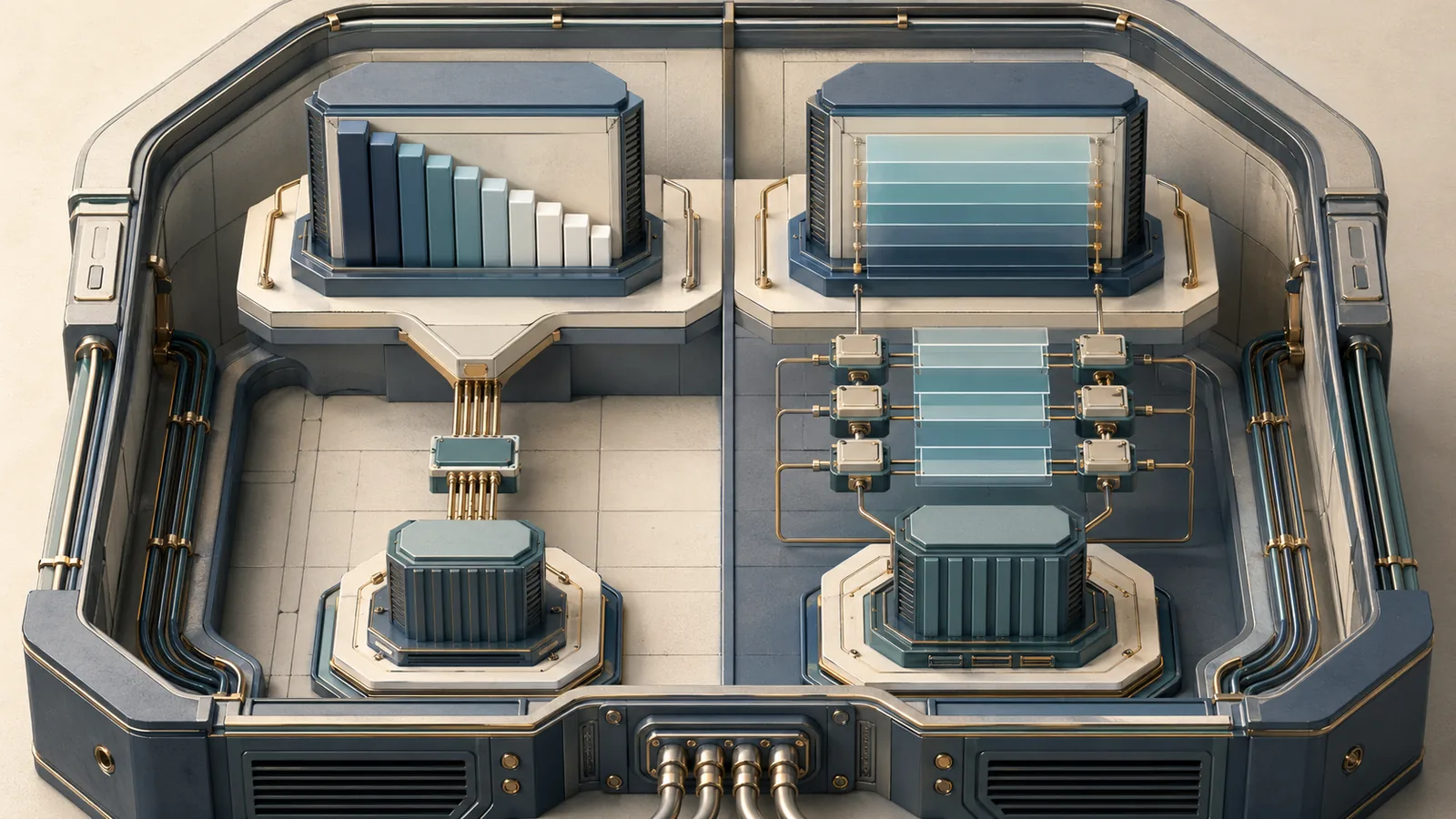
Two fundamentally different training signals drive the two families of knowledge distillation, and choosing between them determines how much of the teacher's internal reasoning the student can recover — not just whether it produces similar output tokens.
What supervision signal each distillation method transfers
The choice between response-based and feature-based knowledge distillation is a choice about where in the teacher you tap the training signal. As NVIDIA's TensorRT Model Optimizer engineering blog states directly: "Response-based knowledge distillation transfers a teacher model's knowledge to a student by training the student to match the teacher's soft output probabilities rather than only hard labels," while "feature-based distillation aligns intermediate hidden activations or feature maps between selected teacher and student layers, commonly using projection layers when dimensions differ." The difference is not stylistic — it determines which gradients flow into the student, from which depth in the network, and what representation structure those gradients impose.
Bottom Line: Response-based KD copies the teacher's output probability distribution over the vocabulary, while feature-based KD copies intermediate hidden activations or feature maps at selected layers. The first supervises the student at the logit level; the second supervises internal representations below the logit level.
Response-based KD: match soft logits, not internals
Response-based knowledge distillation trains the student entirely from the teacher's output distribution — typically the softened token probabilities over the full vocabulary after temperature scaling. The student never observes what happened inside the teacher's attention heads or MLP sublayers; it only sees the final evidence those computations produced.
This matters for two reasons. First, a well-calibrated teacher's soft probabilities encode inter-class relationships that hard labels do not. A teacher assigning 0.6 probability to token A and 0.3 to a semantically related token B is transmitting relational structure that a one-hot label erases. Second, because the supervision path touches only the output projection, this method imposes no constraints on how the student routes information internally — its hidden states are free to form representations that are efficient for its own smaller width and depth.
The practical cost is that the student's representation geometry can diverge substantially from the teacher's, which matters when the downstream application depends on similarity between internal states (retrieval, probing, transfer).
A 2024 arXiv survey on LLM knowledge distillation (arXiv:2402.13116) positions output-based distillation as the most common baseline precisely because it requires only teacher predictions, not internal activations — which is critical when the teacher is a closed API or a hosted endpoint.
Pro Tip: Response-based KD works even when you never have weight access to the teacher. If you can log token-level logits from an inference endpoint (or sample from the teacher's output distribution), you have everything needed to run a full distillation loop. This makes it the natural starting point for any pipeline where the teacher is a proprietary or externally hosted model.
Feature-based KD: align hidden states and intermediate representations
Feature-based KD adds direct alignment losses between paired teacher and student hidden states at intermediate layers. The student's internal representations at selected transformer blocks are explicitly pulled toward the teacher's representations at corresponding blocks — not through an output prediction signal, but through a loss computed directly on the hidden-state tensors.
This creates a denser supervision gradient. Every paired layer generates its own loss term and its own gradient contribution to the student's weights — including weights in early layers that response-based KD would only influence weakly through backpropagation from the final output.
The cost is access and complexity. Teacher activations must be materialized during training, which means the teacher must be resident in memory (or its activations pre-cached), increasing VRAM pressure significantly. Layer pairing requires an explicit mapping between teacher and student layer indices, which is nontrivial when the two models have different depths. Projection heads are required when hidden-state dimensions differ — a 70B teacher with hidden size 8192 cannot be directly compared to a 7B student with hidden size 4096 without a trainable projection that maps one space to the other.
Watch Out: Two failure modes appear together in practice. First, if you select mismatched layer pairs — for example, pairing the teacher's final attention block with the student's middle block — the alignment loss can pull the student's representations toward a semantically incorrect target, degrading both alignment metrics and downstream accuracy. Second, because feature-based KD requires materialized teacher activations, you cannot run it with a black-box teacher accessible only through logit outputs or API sampling. Verify activation access and layer correspondence before committing to this path.
Why the supervision path changes the student's internal representations
The structural reason feature-based KD produces different student representations is that gradients reach earlier layers more directly. In response-based KD, the only signal propagating into the student's early transformer blocks comes from the task or output-matching loss backpropagated through every layer — a signal that weakens with depth and is shaped by the student's own computation path. Feature-based KD injects additional gradient directly at each paired layer, independent of how the student's later layers transform that signal.
NVIDIA's blog frames this explicitly: feature-based distillation is "deeper layer-level supervision," operating below the final vocabulary distribution. A 2024 arXiv survey on LLM KD (arXiv:2402.13116) describes intermediate supervision as transferring knowledge at multiple levels of abstraction rather than only the final response — a description that maps directly to the gradient structure above.
The architecture of the supervision path looks like this:
flowchart LR
    subgraph Teacher ["Teacher (e.g. Llama 3.1 70B)"]
        TL1["Layer 4\nhidden: 8192"]
        TL2["Layer 16\nhidden: 8192"]
        TL3["Layer 32\nhidden: 8192"]
        TLogit["Output logits"]
    end

    subgraph Proj ["Projection Heads"]
        P1["Linear\n8192→4096"]
        P2["Linear\n8192→4096"]
        P3["Linear\n8192→4096"]
    end

    subgraph Student ["Student (e.g. Llama 3.1 7B)"]
        SL1["Layer 2\nhidden: 4096"]
        SL2["Layer 8\nhidden: 4096"]
        SL3["Layer 16\nhidden: 4096"]
        SLogit["Output logits"]
    end

    subgraph Losses ["Loss Terms"]
        FL1["Feature Loss L₁"]
        FL2["Feature Loss L₂"]
        FL3["Feature Loss L₃"]
        RL["Response Loss\n(KL divergence)"]
        TL["Task Loss\n(cross-entropy)"]
    end

    TL1 --> P1 --> FL1 --> SL1
    TL2 --> P2 --> FL2 --> SL2
    TL3 --> P3 --> FL3 --> SL3
    TLogit --> RL --> SLogit
    SLogit --> TL
The diagram captures what competitors' content typically omits: response-based KD contributes exactly one loss path (from teacher logits to student logits), while feature-based KD contributes N additional loss paths through projection heads, one per paired layer. Each feature loss reaches a different depth in the student, constraining intermediate representation geometry that response-based KD never touches. When intermediate losses are dense or aggressively weighted, the student can memorize teacher geometry rather than adapting its own efficient computation structure for its smaller capacity.
How NVIDIA frames distillation inside TensorRT Model Optimizer
NVIDIA TensorRT Model Optimizer frames pruning and knowledge distillation as complementary operations within a unified compression stack rather than alternatives. The official blog states: "This post explains model pruning and knowledge distillation, how they work, and how you can easily apply them to your own models to achieve optimal performance using NVIDIA TensorRT Model Optimizer." The practical implication is that you typically prune to reduce structural size and then use distillation to recover the accuracy that pruning degrades.
Production Note: In TensorRT Model Optimizer deployment workflows, distillation is not a standalone research technique — it is the accuracy-recovery step after structural compression. Prune a model to your target parameter count or layer depth, then run distillation (response-based as the default, feature-based when you need representation recovery) to close the accuracy gap before quantization and TensorRT-LLM export. Treating distillation as a post-pruning refinement step, rather than a primary size-reduction method, keeps the compression pipeline modular and each stage independently debuggable.
Where distillation sits in the compression stack
Pruning and distillation operate on different objects: pruning changes the model's structure by removing parameters, channels, or layers, while distillation changes what the student learns during retraining. The TensorRT Model Optimizer GitHub repository describes the library as "a unified library of state-of-the-art model optimization techniques including quantization, distillation, pruning, speculative decoding and sparsity" — listing them as complementary techniques in a single stack, not mutually exclusive choices.
| Technique | What it changes | Access required | Primary effect |
|---|---|---|---|
| Structured pruning | Model architecture (layers, channels) | Full model weights | Reduces parameter count and FLOP budget |
| Response-based KD | Student output distribution | Teacher logits only | Recovers accuracy after structural changes |
| Feature-based KD | Student + intermediate representations | Teacher activations + logits | Recovers accuracy + representation fidelity |
The practical ordering matters. Pruning first removes redundant structure, leaving a smaller model that fits the target deployment budget. Distillation then repairs the accuracy degradation without adding parameters back. Quantization follows to reduce memory footprint further. Each stage has a distinct input (a trained model) and output (a smaller or lower-precision model), and each can be independently validated.
A critical practical constraint: parameter reduction from pruning does not automatically translate to wall-clock speedup on the target backend. Actual latency improvement depends on whether the pruning pattern maps cleanly to hardware-efficient layouts — which is backend-specific.
What the NVIDIA blog makes concrete about deployable compression
The Mistral-NeMo-Minitron 8B case illustrates the full pipeline concretely. NVIDIA's Minitron blog post describes the 8B base model as produced by width-pruning a 12B base model followed by light retraining with knowledge distillation, and states the result "consistently delivers leading accuracy on nine popular benchmarks." This is the deployment framing: pruning + distillation as a pair that produces a model small enough to serve efficiently while retaining enough accuracy to meet production quality thresholds.
Pro Tip: When choosing between response-based and feature-based KD after pruning, let the deployment constraint drive the decision — not the research aspiration. If your pruned model's logit accuracy is already within acceptable range of the original, response-based KD is sufficient and faster to iterate. If the pruned model's benchmark scores are materially degraded, feature-based KD gives you a second lever by pulling internal representations toward the unpruned teacher. The decision point is the accuracy gap after pruning, not a preference for architectural elegance.
Teacher-student layer pairing and projection heads
The critical engineering decisions in feature-based KD are which layers to pair and how to handle the dimensional mismatch that almost always exists between teacher and student. NVIDIA's blog confirms both requirements: hidden activations are aligned between "selected teacher and student layers," and projection layers are "commonly used when dimensions differ." Neither of these is a detail — layer selection controls which representations the student is forced to mimic, and projection head design determines whether the comparison is even geometrically valid.
flowchart TD
    T4["Teacher Block 4\nH=8192"] -- "select" --> P4["Projection\nLinear(8192→4096)\ntrained jointly"]
    P4 -- "MSE / cosine loss" --> S2["Student Block 2\nH=4096"]

    T16["Teacher Block 16\nH=8192"] -- "select" --> P16["Projection\nLinear(8192→4096)"]
    P16 -- "MSE / cosine loss" --> S8["Student Block 8\nH=4096"]

    T32["Teacher Block 32\nH=8192"] -- "select" --> P32["Projection\nLinear(8192→4096)"]
    P32 -- "MSE / cosine loss" --> S16["Student Block 16\nH=4096"]

    TLogit["Teacher logits"] -- "KL(T‖S) with temperature τ" --> SLogit["Student logits"]
    SLogit -- "cross-entropy" --> TaskLoss["Task loss L_task"]
Selecting which teacher and student layers to align
Layer selection is a heuristic problem without a closed-form solution. The student and teacher have different depths, so a one-to-one correspondence is structurally impossible. The most common strategy is proportional depth mapping: map student layer $i$ to teacher layer (\lfloor i \cdot (D_T / D_S) \rfloor), where (D_T) and (D_S) are teacher and student depths respectively. This preserves the relative position in the network stack, so early-stage syntactic representations pair with early-stage student layers and later-stage semantic representations pair with later ones.
NVIDIA's blog notes that feature-based KD requires "careful layer selection and weighting," and the Minitron arXiv paper confirms that structured pipelines use explicit layer selections rather than indiscriminate alignment of every layer.
Alignment of every layer is not advisable. Aligning only a sparse subset of layers — typically 3 to 6 across the depth of the network — provides supervision at multiple abstraction levels without over-constraining the student's internal organization. Intermediate layers not directly paired remain free to form efficient student-specific representations.
Watch Out: Poor layer mapping over-constrains the student. If you pair a teacher layer that encodes high-level semantic reasoning with a student layer that is structurally an early feature extractor, the alignment loss teaches the student to produce the wrong representation type at the wrong depth. The result is a student that satisfies the alignment objective during training but generalizes poorly on downstream tasks. Always validate paired-layer correspondence by checking that teacher and student layers at the paired indices encode semantically similar content before locking in the mapping.
Why projection heads resolve dimension mismatch
When teacher hidden size (d_T) differs from student hidden size (d_S) — which is true for nearly every practical teacher-student pair — direct comparison of hidden-state tensors is geometrically undefined. A per-layer trainable linear projection (W_i \in \mathbb{R}^{d_T \times d_S}) maps the teacher representation into the student's dimensional space before computing the alignment loss:
$(\mathcal{L}_{\text{feat}}^{(i)} = \left| W_i \, h_T^{(i)} - h_S^{(i)} \right|_2^2)$
where (h_T^{(i)} \in \mathbb{R}^{d_T}) is the teacher hidden state at paired layer $i$, (h_S^{(i)} \in \mathbb{R}^{d_S}) is the student hidden state at its paired layer, and (W_i) is trained jointly with the student. The projection head is not a preprocessing step — it is a trainable component that learns to map teacher geometry into student space, and its gradient contributes to both the student's hidden-state parameters and the projection weights simultaneously.
Without projection heads, engineers sometimes truncate or pad the larger representation to force dimension compatibility. Both approaches are wrong: truncation discards information from the teacher's hidden state arbitrarily, and padding introduces spurious zero-valued dimensions that the alignment loss treats as meaningful. The projection head is the only dimensionally consistent option.
Projection heads add parameters and can themselves become a source of instability. An over-parameterized projection (for example, a multi-layer MLP instead of a single linear map) can absorb the optimization budget and prevent the student's core layers from receiving clean gradient signal.
When paired layers are easy to overfit or destabilize
Instability in feature-based KD typically has two signatures. The first is training loss collapse: the feature alignment losses converge rapidly to near-zero because the projection heads over-adapt to the training distribution rather than guiding the student toward generalizable representations. The second is task-accuracy degradation concurrent with low feature loss — the student mimics the teacher's hidden-state geometry on training examples while failing to generalize, a classic form of overfitting to the supervision signal.
The risk is proportional to the density of supervision. Pairing 12 layers instead of 4, or weighting feature losses 10× higher than task loss, compresses the student's optimization into a much narrower region. The student's own capacity is then spent reproducing teacher geometry rather than solving the downstream task efficiently.
NVIDIA's blog flags this directly: feature-based KD "requires access to internal activations and careful layer selection and weighting." The Minitron paper adopts staged training rather than dense simultaneous supervision, which is the practical mitigation.
Pro Tip: Apply feature losses on a schedule rather than at full weight from step one. A common approach: warm up the student on task loss alone for several hundred steps, then linearly ramp feature loss weights over the next epoch. This gives the student's representations time to stabilize before the alignment pressure activates. If instability persists, reduce the number of paired layers before reducing loss weights — fewer alignment targets is usually more stable than many lightly-weighted ones.
Composite loss design for LLM distillation
A practical knowledge distillation training loop for LLMs combines three loss families: the task loss on ground-truth labels, the response-based output matching loss against teacher logits, and (for feature-based KD) the per-layer hidden-state alignment losses through projection heads. The composite objective is:
$(\mathcal{L}{\text{total}} = \alpha \, \mathcal{L}}} + \beta \, \mathcal{L{\text{response}} + \gamma \sum)$}^{N} \mathcal{L}_{\text{feat}}^{(i)
where (\alpha), (\beta), (\gamma) are scalar weights, $N$ is the number of paired layers, and (\gamma = 0) recovers pure response-based KD. The arXiv survey on LLM KD (arXiv:2402.13116) confirms that multi-term objectives mixing task, output, and representation losses are standard in practice. There is no universal coefficient set — (\alpha), (\beta), and (\gamma) are architecture- and task-specific hyperparameters.
Balancing task loss against distillation loss
The task loss (\mathcal{L}{\text{task}}) — typically cross-entropy against ground-truth labels — is the anchor that keeps the student aligned with the actual objective. Distillation losses ((\mathcal{L})) are auxiliary signals that transfer teacher knowledge, not replacements for the primary objective.}}) and (\mathcal{L}_{\text{feat}
When (\beta) or (\gamma\sum_i) dominate (\alpha), the student optimizes for teacher imitation at the expense of ground-truth performance. This is most visible when the teacher makes systematic errors on the training distribution: a student that perfectly matches the teacher's wrong answers will inherit those errors without correction.
A practical starting point used in the literature (including the regime implied by NVIDIA's compression workflows) is (\alpha \approx 0.5), (\beta \approx 0.5) for response-only KD, with feature loss weights (\gamma) set small relative to (\beta) when enabled — then adjusted based on validation metrics.
Watch Out: Over-weighting imitation losses produces students that are accurate proxies of the teacher on the training distribution but fail to adapt when the deployment distribution shifts. If the teacher is imperfectly calibrated or has domain-specific blind spots, a high-(\beta) student inherits those blind spots more faithfully than a high-(\alpha) student. Monitor task accuracy on a held-out validation set independent of the distillation loss to catch this early.
Temperature, scaling, and gradient signal quality
The response-based loss (\mathcal{L}_{\text{response}}) is computed between temperature-softened teacher and student distributions. Applying temperature (\tau > 1) to both teacher and student logits before computing KL divergence softens the teacher's output distribution, increasing the probability mass on non-top tokens and producing a richer gradient signal:
$(\mathcal{L}{\text{response}} = \tau^2 \cdot D\right) \right))$}}!\left( \sigma!\left(\frac{z_T}{\tau}\right) \Big| \sigma!\left(\frac{z_S}{\tau
where (z_T) and (z_S) are teacher and student logits respectively, (\sigma) is the softmax function, and the (\tau^2) scaling factor compensates for the magnitude reduction introduced by temperature softening — a standard correction from Hinton et al.'s original formulation.
At (\tau = 1), the loss reduces to standard cross-entropy against teacher predictions. At (\tau \gg 1), the distribution becomes nearly uniform and the gradient approaches zero — the student receives a strong noise signal rather than a useful supervision signal. At (\tau < 1), the distribution sharpens toward hard labels, reducing information content. In practice, (\tau \in [2, 6]) spans the useful range for most LLM vocabulary sizes, with higher values beneficial when the teacher is highly confident and you want to spread credit to near-correct tokens.
When feature-based KD is worth the extra complexity
Feature-based KD adds engineering cost across three dimensions: it requires teacher activation access during training (ruling out black-box teachers), it demands layer pairing and projection head design, and it introduces additional loss terms that interact with task and response objectives. NVIDIA states directly that it "provides deeper layer-level supervision but requires access to teacher activations and careful layer matching to avoid instability." The question is when that cost is justified by accuracy or representation gains.
| Condition | Response-based KD | Feature-based KD |
|---|---|---|
| Teacher accessible via logits/API only | ✅ Works | ❌ Not possible |
| Teacher and student same architecture family | ✅ Sufficient | ✅ Useful — easy pairing |
| Large depth gap (e.g., 80L → 16L) | ✅ Viable | ⚠️ Hard layer mapping |
| Representation fidelity required (retrieval, probing) | ⚠️ Limited | ✅ Primary advantage |
| Post-pruning accuracy recovery, moderate gap | ✅ Often sufficient | ✅ Better if gap is large |
| Engineering team bandwidth constrained | ✅ Preferred | ⚠️ Adds iteration cost |
| Student trained with FSDP / DeepSpeed across nodes | ✅ Compatible | ⚠️ Teacher activation sync adds memory cost |
Use cases where hidden-state supervision pays off
Hidden-state supervision earns its complexity premium in specific scenarios where matching teacher output distributions is structurally insufficient.
The clearest case is large teacher-student capacity gaps combined with architectural similarity. When distilling a 70B model (hidden size 8192, 80 layers) into a 7B model (hidden size 4096, 32 layers) within the same model family — say, Llama 3.1 70B to Llama 3.1 7B — layer correspondence is well-defined and the student's hidden states are directly comparable to teacher hidden states after projection. Feature-based KD injects gradient into the 7B model's earlier layers with a directional signal from the 70B teacher, which response-based KD cannot match.
The second case is post-pruning recovery when the pruning operation removed a large fraction of the model's internal structure. Pruning that removes entire layers or reduces hidden width dramatically can shift the student's internal representations far from the teacher's. Output matching can repair benchmark scores on simple tasks but leaves internal geometry fragmented, which degrades performance on tasks that depend on representation coherence — reasoning chains, multi-hop retrieval, structured generation.
The third case is distillation pipelines producing students that will be further fine-tuned or probed. Feature-based KD gives the student's representations a stronger structural prior from the teacher, which tends to reduce catastrophic forgetting in subsequent fine-tuning.
Bottom Line: Feature-based KD tends to win in three scenarios: (1) large teacher-student capacity gaps within the same model family where layer pairing is tractable; (2) post-pruning recovery where the internal representation structure has been substantially disrupted; (3) pipelines where the student will be subsequently fine-tuned or probed and representation coherence matters. Outside these scenarios, the added complexity rarely pays.
Cases where response-only distillation is the safer default
Response-based knowledge distillation is the correct starting point for most practical compression pipelines. It requires only teacher logits, which means it is compatible with hosted or API-accessible teachers — a decisive advantage when the teacher weights are not available. It eliminates projection head design, layer pairing, and activation memory overhead, which shortens iteration cycles significantly.
The arXiv survey on LLM KD (arXiv:2402.13116) documents output-based distillation as the most common baseline across the literature precisely because of this operational simplicity. Many production teams that have run both methods report that response-based KD recovers the majority of accuracy in post-pruning recovery — the marginal gain from adding feature losses is real but often small relative to the engineering investment.
Response-based KD also fails more gracefully. If temperature scaling is wrong or the teacher is miscalibrated, the failure mode is a student with suboptimal soft-target matching — diagnosable and correctable. Feature-based KD failures (layer mismatch, over-constrained representations, instability from dense losses) are harder to diagnose because they manifest as subtle representation distortions that may not appear in the training loss.
Pro Tip: Run response-based KD to completion first and measure the post-distillation benchmark gap. If the gap is within your accuracy budget, ship it — the lower operational friction of a response-only pipeline reduces failure modes and simplifies debugging in production. Escalate to feature-based KD only when the benchmark evidence shows that output matching alone is insufficient. This "response-first" default is consistent with how NVIDIA frames distillation as a practical tool: get the simpler method working before adding the complex one.
Practical signals to watch during training and evaluation
Distillation training produces multiple loss curves — task loss, response loss, per-layer feature losses if enabled — and none of them alone is sufficient to evaluate whether the student is learning the right thing. The 2024 arXiv survey on LLM KD (arXiv:2402.13116) recommends tracking task metrics, distillation losses, and retention indicators together. NVIDIA's blog adds that careful layer selection and weighting implies alignment quality is itself a training signal requiring active monitoring.
| Signal | What it measures | Warning sign |
|---|---|---|
| Task validation loss | Student ground-truth accuracy | Stagnation while distillation loss falls |
| Response KL loss | Output distribution alignment to teacher | Rapid early collapse (potential mode collapse) |
| Feature MSE per layer | Hidden-state alignment at each paired layer | Loss diverges on later layers but not earlier |
| Benchmark accuracy (MMLU, GPQA) | End-task retention | Drops vs teacher after distillation |
| Gradient norm per layer | Training stability | Spikes in early student layers during feature KD |
Accuracy retention vs representation fidelity
Better hidden-state alignment does not automatically produce better downstream accuracy. This is the most common misinterpretation in feature-based KD results. A student can achieve low feature MSE on all paired layers while still underperforming on MMLU or GPQA relative to a response-only distilled student — because the projection heads absorb representational variation that the student's downstream task computation needed.
The Minitron paper (arXiv:2408.11796) shows that pruning plus distillation pipelines can preserve or improve benchmark performance relative to larger baselines, but the validation methodology is benchmark-level accuracy, not representation-level alignment metrics. The Mistral-NeMo-Minitron 8B result — "leading accuracy on nine popular benchmarks" after pruning from 12B and distillation recovery — is evidence for the end-to-end pipeline, not for representation alignment as a proxy for downstream quality.
Watch Out: Do not conclude that feature-based KD is "working" because feature losses are decreasing. Always validate against held-out benchmark tasks. A student with excellent feature alignment but degraded MMLU accuracy compared to a response-only distilled baseline is evidence of over-constraint, not progress. Representation fidelity metrics are diagnostics, not success criteria.
What to report when comparing compressed models
Benchmark accuracy after compression is the minimum reportable metric, but it is not sufficient for engineering decisions. Downstream stakeholders need the full compression profile: parameter count reduction, memory footprint before and after quantization, and — most critically — latency or throughput on the target runtime stack.
Parameter count reduction from pruning does not guarantee proportional latency improvement. Wall-clock speedup is backend-dependent: a width-pruned model may achieve near-linear speedup on TensorRT-LLM with optimized kernels but show minimal improvement on a CPU runtime that cannot exploit the structural sparsity. Report latency on the specific deployment target (TensorRT-LLM, vLLM, Triton), not FLOP reduction.
Pro Tip: When presenting distillation results, report at minimum: (1) benchmark accuracy on the target task suite (e.g., MMLU, GPQA) for both teacher and student; (2) student parameter count and memory footprint; (3) inference latency or tokens/second on the target backend at your production batch size. Parameter count alone is a misleading proxy for deployment performance. The TensorRT Model Optimizer pipeline is explicitly deployment-oriented — accuracy numbers without latency numbers are incomplete for production decisions.
FAQ
What is the difference between feature-based and response-based knowledge distillation?
Response-based KD trains the student to match the teacher's softened output token probabilities — the supervision signal is the teacher's vocabulary distribution after the final projection layer. Feature-based KD adds direct alignment losses between teacher and student hidden states at selected intermediate layers, injecting supervision below the logit level. The key practical difference: response-based KD needs only teacher logits, while feature-based KD requires teacher activations during training.
Is feature-based knowledge distillation better than response-based distillation?
Neither method dominates in all conditions. Feature-based KD provides richer supervision and tends to preserve internal representation structure better — which matters in large capacity-gap scenarios, post-aggressive-pruning recovery, and downstream fine-tuning pipelines. Response-based KD is simpler, more compatible with black-box or API-hosted teachers, and fails more gracefully. The right default is response-based KD; escalate to feature-based KD when benchmark evidence after response-only distillation shows an insufficient accuracy gap recovery.
Why do you need projection layers in feature-based distillation?
Teacher and student hidden-state dimensions almost always differ. A Llama 3.1 70B teacher uses hidden size 8192; a Llama 3.1 7B student uses 4096. Directly computing an alignment loss between vectors of different dimensions is geometrically undefined. A trained linear projection (W_i \in \mathbb{R}^{d_T \times d_S}) maps the teacher representation to the student's space before the loss is computed. Truncating or padding hidden states as an alternative is incorrect: truncation discards information arbitrarily, and padding introduces spurious dimensions. The projection head is not optional when dimensions differ.
Can knowledge distillation and pruning be used together?
Yes — NVIDIA frames them as complementary stages in the TensorRT Model Optimizer compression stack, not alternatives. The standard pipeline is: prune the model to the target architecture (removing layers, channels, or heads), then apply distillation to recover accuracy that pruning degrades, then quantize for deployment. The Mistral-NeMo-Minitron 8B model was produced by exactly this sequence: width-pruning a 12B model, then distillation recovery, yielding a model that achieves leading accuracy on nine benchmarks at 8B parameters.
Which training frameworks support feature-based KD for large LLMs?
Feature-based KD runs on standard PyTorch training infrastructure — Hugging Face Trainer, DeepSpeed ZeRO, and FSDP all support it, but you need to hook into intermediate layers to materialize teacher activations. NVIDIA's Model Optimizer library provides a productized implementation within TensorRT Model Optimizer workflows. With DeepSpeed or FSDP, teacher activation materialization across distributed workers adds memory pressure; verify that the combined teacher + student activation buffer fits within your GPU memory budget before running multi-node feature-based KD.
Does better hidden-state alignment guarantee better benchmark accuracy?
No. Alignment loss and downstream task accuracy are correlated objectives, not equivalent ones. A student can achieve low feature MSE across all paired layers while still underperforming on MMLU or GPQA compared to a simpler response-only baseline. Always validate against task benchmarks — alignment metrics are diagnostics, not success criteria.
Sources & References
- Pruning and Distilling LLMs Using NVIDIA TensorRT Model Optimizer — Primary source: NVIDIA engineering blog defining response-based and feature-based KD, framing pruning and distillation as complementary compression techniques in TensorRT Model Optimizer
- Mistral-NeMo-Minitron 8B Foundation Model Delivers Unparalleled Accuracy — NVIDIA technical blog documenting the width-pruning + distillation pipeline used to produce Minitron 8B
- NVIDIA Model Optimizer — GitHub Repository — Official NVIDIA repository for the unified optimization library including quantization, distillation, pruning, speculative decoding, and sparsity
- A Survey on Knowledge Distillation of Large Language Models (arXiv:2402.13116) — 2024 arXiv survey covering output-based and feature-based distillation methods, composite objectives, and temperature scaling for LLMs
- Compact Language Models via Pruning and Knowledge Distillation (arXiv:2408.11796) — Minitron technical paper documenting structured pruning plus distillation pipelines and layer selection strategies
Keywords: knowledge distillation, feature-based KD, response-based KD, TensorRT Model Optimizer, NVIDIA Model Optimizer, Llama 3.1 70B, Llama 3.1 7B, Qwen3-8B, Qwen3-6B, PyTorch, Hugging Face Trainer, DeepSpeed, FSDP, MMLU, GPQA