How We Compared MHA, GQA, and MQA
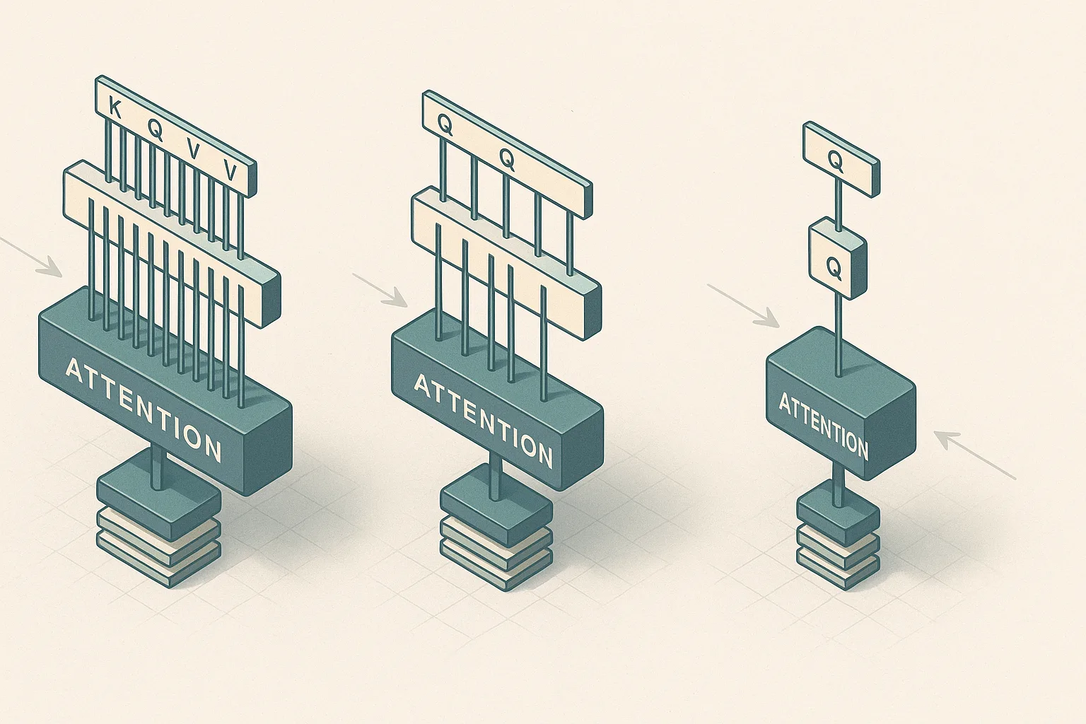
The three attention variants differ in exactly one structural dimension: how many key/value head projections exist relative to query heads. Multi-head attention (MHA) gives every query head its own dedicated K and V projection. Multi-query attention (MQA) collapses all query heads onto a single shared K/V pair. Grouped-query attention (GQA) places G groups of query heads, each group sharing one K/V pair, and thereby spans the full continuum: as the GQA paper (arXiv:2305.13245) defines it, GQA-1 is exactly MQA and GQA-H (groups equal to number of heads) is exactly MHA.
"Grouped-query attention divides query heads into G groups, each of which shares a single key head and value head." — GQA paper, arXiv:2305.13245
| Variant | KV-head count | KV-cache footprint | Decode bandwidth pressure | Head-sharing degree |
|---|---|---|---|---|
| MHA | H (one per query head) | Highest (1× per head) | Highest | None — each head independent |
| GQA | G (1 < G < H) | Proportional to G/H of MHA | Scales with G/H | Moderate — H/G query heads per KV |
| MQA | 1 (shared across all) | Lowest (1/H of MHA) | Lowest | Maximum — all heads share one KV |
Because GQA-1 equals MQA and GQA-H equals MHA, any comparison table must specify group count rather than treating GQA as a single fixed design. The structural difference between these variants does not change parameter count in the feed-forward stack, positional encoding, or layer count — it only changes the dimensionality of K and V projections and therefore the cache footprint those projections generate at inference time.
Comparison criteria that matter in long-context decoding
The decisive constraint during autoregressive decoding is not compute throughput but memory bandwidth for loading keys and values. The GQA paper frames this directly: "This paper focuses on ameliorating the memory bandwidth overhead from loading keys and values." That overhead compounds with sequence length: "This overhead is most important when generating longer sequences, for which quality is inherently difficult to evaluate."
The scoring criteria that matter for this comparison are:
- KV-cache bytes per token — how much VRAM each generated token occupies across all layers
- Memory traffic per decode step — how many bytes the GPU must read from HBM to complete one autoregressive step
- Quality retention — how much task performance degrades relative to MHA as head sharing increases
- Latency sensitivity — how decode throughput responds to bandwidth reduction from fewer KV heads
Pro Tip: When sizing a long-context serving stack — 32k tokens and beyond — KV-cache residency determines concurrent batch capacity more directly than model parameter count does. GQA and MQA cut cache per sequence, which raises the number of sequences that fit in a fixed VRAM budget. PagedAttention in vLLM manages allocation of those KV blocks efficiently, but it operates on top of whatever cache size the attention design generates; it does not reduce that size.
What we hold constant across the three attention variants
A fair comparison holds constant: hidden size ((d_{model})), number of query heads (H), head dimension ((d_h = d_{model}/H)), number of transformer layers (L), context length (S), dtype, the feed-forward stack, and positional encoding. Changing any of these confounds cache and latency deltas with unrelated architectural decisions.
The GQA paper's equivalence statements imply exactly this: the only variable is the number of KV heads (which equals G, the group count). Llama-family models using GQA confirm this in practice — the broader autoregressive transformer design is kept intact while KV-head count is reduced for inference scalability, as shown in model metadata for Llama 3.2.
Watch Out: RoPE (rotary position embeddings) is applied to query and key projections, not to values. Switching attention variant does not change RoPE behavior, but if you change head dimension during an architecture experiment — for example, by merging heads — you will change RoPE's effective frequency spectrum and contaminate the comparison. Keep (d_h) fixed. Similarly, if you fine-tune from an MHA checkpoint and compare against a from-scratch GQA model, you are measuring checkpoint transfer quality, not architecture quality.
At-a-glance comparison of KV-cache trade-offs
GQA reduces KV-cache memory because it directly reduces the number of K and V tensors that must be materialized and stored per token. Under MHA, every one of the H heads maintains its own K and V projection for every token in the context window. GQA replaces H separate KV pairs with G shared ones, where G < H. MQA takes this to the extreme with G = 1.
| Variant | KV heads per layer | Per-token KV traffic (relative) | Head-sharing degree | Quality vs MHA | Typical production use |
|---|---|---|---|---|---|
| MHA | H | 1.0× | None — each head independent | Reference | Encoder models, smaller decoders, quality-first research |
| GQA (G = H/4) | H/4 | 0.25× | Moderate — H/G query heads per KV | Close to MHA | Llama 3.1 70B, Llama 3.2, most 2024–2025 production LLMs |
| GQA (G = H/8) | H/8 | 0.125× | Higher sharing than H/4 | Moderate degradation | Aggressive throughput targets, very long context |
| MQA | 1 | 1/H × | Maximum — all heads share one KV | Noticeable degradation | Latency-critical edge, extreme cache pressure |
The KV-cache footprint reduction is proportional to the ratio of KV heads to query heads. This is not a free lunch: as G decreases toward 1, each KV head must serve more query heads, reducing the representational diversity available in the attention output. The GQA paper reports that "uptrained GQA achieves quality close to multi-head attention with comparable speed to MQA" — meaning mid-range group counts preserve most of the quality while recovering most of the bandwidth savings.
KV-cache footprint per generated token
For a model with $L$ layers, (H_q) query heads, (H_{kv}) KV heads (equal to the number of groups G), head dimension (d_h), sequence length $S$, and a dtype of size $b$ bytes (e.g., $b = 2$ for bfloat16), the KV-cache size for a single sequence is:
$(\text{KV-cache}(S) = 2 \cdot L \cdot H_{kv} \cdot d_h \cdot S \cdot b \text{ bytes})$
The factor of 2 accounts for both K and V tensors. For MHA, (H_{kv} = H_q). For GQA, (H_{kv} = G) where (1 \leq G \leq H_q). For MQA, (H_{kv} = 1).
These values scale linearly with sequence length and with the number of KV heads, so the useful comparison is the ratio rather than a universal GB figure. The exact byte count depends on the model's layer count, head dimension, and serving dtype.
"GQA-1, with a single group and therefore single key and value head, is equivalent to MQA, while GQA-H, with groups equal to number of heads, is equivalent to MHA." — GQA paper, arXiv:2305.13245
These numbers are illustrative; the actual values require your model's specific layer count, KV-head count, head dimension, and serving dtype. Do not use a single universal number across architectures.
Decode-time memory bandwidth pressure
At each autoregressive decode step, the GPU reads the entire KV cache for the current sequence from HBM to compute attention. With a context of $S$ tokens, a single decode step requires:
$(\text{Bytes read per step} = 2 \cdot L \cdot H_{kv} \cdot d_h \cdot S \cdot b)$
This is the same expression as total cache size — every step reads the full cache. Under MHA, this saturates memory bandwidth proportionally to (H_q). Under GQA with (H_{kv} = G), the read burden scales down by (G / H_q). Under MQA, it scales down to (1 / H_q) of MHA.
This bandwidth dependency is the reason attention-variant choice dominates decode-throughput decisions on bandwidth-limited hardware. The NVIDIA H200 delivers 4.8 TB/s of HBM3e bandwidth, which is materially higher than H100-class configurations, but even on Hopper hardware a 70B MHA model at 32k context with large batch sizes can saturate memory reads before saturating compute. The FlashAttention-3 paper notes that FlashAttention-2 achieved only 35% utilization on H100, which reveals that even with tiled kernel optimizations, attention on Hopper-class hardware can remain memory-bound. Reducing (H_{kv}) through GQA or MQA directly cuts the bytes-per-step and shifts the model toward the compute-bound regime where arithmetic intensity improves.
NVIDIA H100 note: The H200 datasheet gives a concrete 4.8 TB/s figure; the H100 SXM5 specification (3.35 TB/s HBM3) was not the primary retrieved source here. Use vendor datasheets for hardware-specific planning rather than estimates derived from this comparison.
Multi-head attention: maximum capacity, maximum KV cost
MHA is the upper-bound reference in the attention design space. Every query head attends over its own independent K and V projections — no sharing, no approximation, full representational capacity. In the GQA framework this is GQA-H, with groups equal to the number of heads.
Production Note: MHA remains the right choice when head-level specialization is non-negotiable: encoder models used for retrieval or reranking where query-document interaction patterns benefit from diverse attention heads, smaller decoder models (sub-7B) where the absolute cache size is manageable, and research baselines where you need a clean quality ceiling before ablating head-sharing. If VRAM is not a serving constraint at your target context length, there is no architectural reason to move away from MHA.
Where MHA preserves quality that sharing can erode
MHA avoids the "quality degradation issues observed with MQA" by construction — each head retains an independent K and V projection that can specialize to attend over different token relationships. Tasks that depend on this specialization — multi-step reasoning chains, structured output with complex cross-references, fine-tuned models where specific heads encode domain-specific patterns — can show measurable regression when those heads are merged.
Watch Out: If you plan to fine-tune from an MHA pretrained checkpoint and then evaluate on long-context or complex reasoning benchmarks, be cautious about uptrained KV-head reduction. The GQA paper's uptraining recipe requires retraining a fraction of pretraining compute; a short fine-tune may not sufficiently redistribute the representational load across the reduced head count. Quality drift is workload-dependent and likely largest where specialized attention heads carry task-critical information.
Why MHA becomes expensive at long context
Cache growth under MHA is linear in sequence length and scales with the full head count. At long context, even a single inference sequence for a 70B model can consume substantial KV cache, crowding out other sequences from the batch. This is not a theoretical concern: "This overhead is most important when generating longer sequences."
The serving consequence is lower concurrency. When each sequence holds a large cache reservation, the serving engine can run fewer simultaneous sequences before exhausting VRAM — directly reducing tokens-per-second-per-GPU at the fleet level.
Pro Tip: At context lengths above 32k, MHA cache pressure can reduce effective batch size to single digits on a single H100. If your throughput target requires batches of 16 or more sequences at long context, MHA will force either tensor parallelism across multiple GPUs (increasing NCCL communication overhead on InfiniBand) or a switch to GQA/MQA. Quantify your batch target and context distribution before committing to MHA at scale.
Grouped-query attention: the middle ground that modern LLMs favor
GQA is not a single architecture — it is a parameterized family indexed by group count G. The central empirical claim from the GQA paper is precise: "We show that uptrained GQA achieves quality close to multi-head attention with comparable speed to MQA." This positions GQA on a better quality-latency Pareto frontier than MQA while substantially cutting the cache cost of MHA.
| Group count G | KV heads (H=32) | Cache vs MHA | Quality vs MHA | Decode speed vs MQA | Quality-latency trade-off |
|---|---|---|---|---|---|
| 32 (= MHA) | 32 | 1.0× | Reference | Slowest | Maximum quality, weakest serving efficiency |
| 16 | 16 | 0.5× | Very close | Moderate gain | Slightly lower quality, clearly better latency |
| 8 | 8 | 0.25× | Close (GQA paper regime) | Near MQA | Best balance for most long-context serving |
| 4 | 4 | 0.125× | Moderate degradation | Near MQA | Strong bandwidth relief, more quality risk |
| 1 (= MQA) | 1 | 1/32× | Noticeable degradation | Fastest | Lowest cache cost, highest quality risk |
The table uses H=32 as a concrete example. Quality columns are directional, not absolute — the paper benchmarks the G=8 regime for a 30B-scale model and finds acceptable degradation; exact deltas depend on task type and training budget for uptraining.
How grouping query heads changes the KV-cache shape
With (H_q) query heads and $G$ groups, GQA assigns (H_q / G) query heads to each group, and each group maintains exactly one K projection and one V projection. The symbolic relationships follow directly:
$(H_{kv} = G, \quad \text{where} \quad 1 \leq G \leq H_q)$
$(G = 1 \Rightarrow H_{kv} = 1 \quad \text{(MQA)})$
$(G = H_q \Rightarrow H_{kv} = H_q \quad \text{(MHA)})$
For any intermediate G, the attention computation for group $g$ is:
$(\text{Attention}_g(Q_g, K_g, V_g) = \text{softmax}!\left(\frac{Q_g K_g^T}{\sqrt{d_h}}\right) V_g)$
where (Q_g \in \mathbb{R}^{(H_q/G) \times S \times d_h}) are the query heads assigned to group $g$, and (K_g, V_g \in \mathbb{R}^{S \times d_h}) are the single shared K and V for that group. The KV-cache shape per layer becomes ([2, S, G, d_h]) instead of ([2, S, H_q, d_h]) under MHA. The savings ratio is exactly (G / H_q).
How to choose a GQA group size for a custom architecture
DecisionMatrix:
| Context length | Throughput priority | Quality tolerance | Recommended G (for H=32) |
|---|---|---|---|
| ≤ 8k | Latency-first | Low (tight quality budget) | 16–32 (lean toward MHA) |
| ≤ 8k | Throughput-first | Moderate | 8 |
| 8k–128k | Throughput-first | Moderate | 4–8 |
| 8k–128k | Latency-first | Low | 8–16 |
| > 128k | Throughput-first | Moderate–high | 2–4 |
| > 128k | Quality-first | Low | 8 minimum; benchmark carefully |
Group size selection is a function of four interacting variables: context length, throughput target, quality tolerance, and KV-cache budget. No single published threshold covers all architectures, but the following decision framework reflects the GQA paper's design intent and production deployment patterns.
Start at G = H/4 (e.g., G=8 for H=32) as your initial candidate — this is the regime the GQA paper validates most directly and the regime used by Llama-class models. Then measure perplexity and task accuracy against your MHA baseline. If bandwidth is still the bottleneck and quality delta is acceptable, step down to G = H/8. Do not step to MQA (G=1) without explicit benchmarking; the quality degradation is nonlinear near the single-group extreme.
Why GQA is common in Llama-family models and other long-context stacks
Llama 3.2 uses GQA across all model sizes specifically for inference scalability. The Llama 3.2 model metadata states: "All model versions use Grouped-Query Attention (GQA) for improved inference scalability." These are production decisions driven by the bandwidth-quality trade-off the GQA paper quantifies — not a conservative choice waiting for something better.
Pro Tip: For production LLMs served at scale on H100 or H200 hardware, GQA at G = H/4 to H/8 is the empirically validated starting point in 2025–2026. The bandwidth reduction cuts per-sequence cache cost enough to allow continuous batching at long context without tensor-parallelism overhead on every request. If your model needs to run on a single GPU at 128k context with non-trivial batch sizes, GQA is not optional — it is an operational requirement.
Multi-query attention: maximum cache savings, maximum sharing
MQA is the single-group extreme: GQA-1 with one K/V pair shared across all (H_q) query heads. The KV-cache scales with one key/value set per layer rather than one per head, reducing cache footprint by a factor of (H_q) relative to MHA. The bandwidth reduction at decode time is proportionally identical.
Production Note: MQA makes sense when the KV-cache budget is a hard constraint that GQA cannot satisfy. Specific scenarios: on-device inference where DRAM capacity is measured in gigabytes rather than tens of gigabytes; batch-serving architectures that must maximize concurrent sequence count above all else; draft models in speculative decoding pipelines where the draft model runs at high throughput and quality requirements are deliberately relaxed; and experiments or ablations where you need to establish the bandwidth floor before choosing a GQA group count.
Why a single shared K/V head changes inference economics
With (H_{kv} = 1) under MQA, the per-layer KV-cache for a sequence of length $S$ is:
$(\text{KV-cache}_{\text{MQA}} = 2 \cdot L \cdot 1 \cdot d_h \cdot S \cdot b = \frac{2 \cdot L \cdot d_h \cdot S \cdot b}{1})$
Compare to MHA where the same expression multiplies by (H_q). The per-decode-step read cost follows the same ratio — MQA reads (1/H_q) of the KV bytes that MHA reads at each step. For H_q = 32, that is a 32× reduction in KV-read traffic per step. This shifts the arithmetic intensity of the attention operation substantially and can push the computation from memory-bound toward compute-bound — a favorable shift for throughput on high-FLOP hardware.
The savings are inference-side: MQA does not materially reduce training compute, which depends on the full query-key dot-product over all heads.
Where MQA tends to lose compared with GQA
The GQA paper is explicit that it was designed to address "quality degradation issues observed with MQA." A single shared K/V pair must serve all (H_q) query heads simultaneously, eliminating the head-level diversity in key and value representations. Tasks where attention heads specialize — long-context retrieval, multi-hop reasoning, instruction-following with fine-grained constraints — are most sensitive to this collapse.
Watch Out: MQA's quality loss is not uniform across task types or model scales. Larger models with more query heads per KV head face a steeper capacity reduction. Fine-tuned models that have developed head specialization through task-specific training are at higher risk than base pretrained models. If you are evaluating MQA for a production use case, benchmark on your specific task distribution — general-purpose perplexity metrics will underestimate the degradation on structured outputs or multi-turn instruction tasks.
Benchmarks and serving implications for long-context systems
The GQA paper's central result sets the quantitative anchor: uptrained GQA achieves quality close to MHA while matching MQA's decode speed. The following table translates that framework into serving-relevant metrics with concrete reference points from the sourced hardware and serving literature.
| Metric | MHA | GQA (G=H/4) | MQA | Notes |
|---|---|---|---|---|
| KV-cache per token (relative) | 1.0× | 0.25× | 1/H × | Formula: (2 \cdot L \cdot H_{kv} \cdot d_h \cdot b) |
| KV read bytes per decode step (relative) | 1.0× | 0.25× | 1/H × | Linear in (H_{kv}) |
| Quality vs MHA (literature) | Reference | Close (GQA paper) | Noticeable drop | Task-dependent |
| Max sequences at 32k ctx (relative) | 1× | ~4× | ~H× | Scales inversely with cache |
| H200 bandwidth headroom | Lowest | Moderate | Highest | H200: 4.8 TB/s per NVIDIA |
| FA3 kernel utilization on H100 (baseline) | 35%* | 35%* | 35%* | *FA2 figure, FA3 improves on this |
The bandwidth headroom column reflects that reducing (H_{kv}) decreases the per-step read volume, giving the attention kernel more arithmetic work per byte and moving it closer to the compute-bound regime where FlashAttention-3's improved pipeline efficiency applies. The 35% H100 utilization figure for FlashAttention-2 from the FA3 paper illustrates the baseline — FA3 improves on this, but the structural KV read volume from MHA remains the first-order problem.
For production systems, the serving-relevant outcome is concurrent batch capacity. At 32k context, the ~4× cache reduction from GQA (G=H/4) versus MHA translates directly to ~4× more sequences fitting in the same VRAM budget, which at constant request arrival rate means ~4× higher sustainable throughput before autoscaling is needed.
How PagedAttention changes the serving picture
PagedAttention in vLLM manages KV memory as fixed-size blocks allocated on demand rather than contiguously pre-reserved. This eliminates internal fragmentation and allows multiple sequences to cohabitate in the same physical VRAM pages, significantly improving memory utilization efficiency. However, PagedAttention operates at the allocation layer — it does not change the number of K and V tensors that GQA, MQA, or MHA require per token.
The vLLM PagedAttention documentation now carries an explicit caveat: "Warning. This is a historical document based on the original paper for vLLM. It no longer describes the code used in vLLM today." Current vLLM uses its own multi-head query attention kernel implementation that has evolved beyond the original description. vLLM supports GQA natively — serving Llama-family GQA models is a first-class use case.
Pro Tip: PagedAttention improves how KV blocks are stored and shared (e.g., prefix caching), but it does not shrink those blocks. A GQA model with 8 KV heads will have blocks that are 4× smaller than the equivalent MHA model with 32 KV heads. Switching from MHA to GQA before deploying with PagedAttention multiplies the benefits: smaller blocks mean more concurrent sequences fit in the paged pool. If you are migrating a serving stack to vLLM, the architecture decision and the serving-engine decision are complementary, not substitutes.
FlashAttention 3, kernel efficiency, and what it does not fix
FlashAttention-3 introduces asynchronous execution of GEMM and softmax operations on Hopper GPUs, overlapping compute and memory access to reduce the effective bandwidth bottleneck. The FA3 paper targets the gap that FA2 left open — only 35% H100 utilization — by improving Hopper kernel efficiency. For long-context inference, FA3 reduces the latency penalty of attending over long sequences.
What FA3 does not change: the number of KV heads that must be materialized and loaded from HBM. A 32-head MHA model still materializes 32 times the KV tensors of an MQA model. FA3 makes the kernel more efficient at processing those reads, but it cannot eliminate them.
Watch Out: Switching to FlashAttention-3 on H100 or H200 hardware will improve attention kernel throughput, but it will not resolve a VRAM capacity problem caused by MHA's cache footprint. If your serving bottleneck is total cache size rather than per-kernel compute time, FA3 alone is insufficient. You need a lower-(H_{kv}) architecture — GQA or MQA — to address the structural problem. FA3 and reduced-head attention are complementary optimizations that address different parts of the decode-time budget.
Decision matrix for custom LLM architecture choices
The choice between MHA, GQA, and MQA reduces to three interacting constraints: quality tolerance, context length, and KV-cache budget. The GQA paper establishes the theoretical framing; production deployment of Llama 3.1 70B, Llama 3.2, and similar models confirms the practical default.
| Scenario | Context length | Quality requirement | Throughput priority | Recommended choice |
|---|---|---|---|---|
| Quality-first research model | ≤ 8k | Maximum | Low | MHA |
| Production chat, moderate context | 8k–32k | High | High | GQA (G = H/4 to H/8) |
| Long-context RAG / agents | 32k–128k | High | High | GQA (G = H/4, benchmark G = H/8) |
| Speculative decoding draft model | Any | Relaxed | Maximum | MQA |
| On-device inference | ≤ 8k | Moderate | Cache-constrained | MQA or GQA (G small) |
| Fine-tuned domain specialist | ≤ 32k | High (head specialization) | Moderate | GQA (G = H/4) or MHA |
Choose MHA when head-level capacity matters more than memory savings
MHA is correct when representational diversity across heads is the binding constraint: encoder models where every layer's attention pattern is critical, small decoder models (under 7B parameters) where the absolute cache footprint at target context lengths fits in available VRAM without pressure, and research baselines where you need the quality ceiling before ablating architecture choices.
Production Note: MHA is not a legacy default that GQA has universally obsoleted. For models deployed at short to medium context (under 8k tokens) on hardware with sufficient VRAM, MHA preserves full head-level freedom at no practical serving cost. The decision to move away from MHA should be driven by a measured VRAM constraint or throughput requirement, not by default adoption of whatever the largest public model uses.
Choose GQA when you need the best balance for production LLMs
GQA at G = H/4 to H/8 is the empirically grounded default for production LLMs serving long-context workloads in 2025–2026. It reaches quality close to MHA while recovering most of MQA's bandwidth advantage. Llama 3.1 70B and Llama 3.2 both use GQA for exactly this reason.
Pro Tip: For long-context workloads on H100/H200 hardware, treat G = H/4 as the starting point and benchmark downward. The quality-bandwidth curve is concave — the first reduction from MHA to GQA (G=H/4) recovers most of the bandwidth savings with minimal quality loss; subsequent reductions toward MQA yield diminishing quality returns for each incremental bandwidth gain.
Choose MQA when cache pressure dominates everything else
MQA makes sense when the serving constraint is a hard KV-cache ceiling that GQA cannot meet: speculative decoding draft models where quality is deliberately subordinate to speed, on-device inference with tight DRAM constraints, or architectures where you have experimentally confirmed that the quality penalty is acceptable for your specific task distribution.
Watch Out: MQA's quality degradation is not uniformly distributed across workloads. Accepting MQA without task-specific benchmarking is a structural risk. A model that shows acceptable perplexity under MQA on a general benchmark may fail noticeably on structured output, multi-step reasoning, or fine-grained instruction following. Measure on your actual task before committing MQA to production.
Questions readers ask about GQA, MQA, and MHA
What is the difference between multi-head attention and grouped query attention?
MHA gives every query head its own K and V projections. GQA groups query heads so that each group shares one K and one V projection, reducing the number of KV heads from H to G (where G < H). The structural result is a smaller KV cache and lower decode-time memory bandwidth, at a modest quality cost that scales with how aggressively G is reduced below H.
Is grouped query attention better than multi-query attention?
For most production use cases, yes. The GQA paper demonstrates that uptrained GQA reaches quality close to MHA while matching MQA's speed — placing it on a better quality-latency trade-off than MQA alone. MQA's additional cache savings are real but come with higher quality risk. The exception is scenarios where the cache budget is so tight that only MQA's single-KV-head design fits the constraint.
Why does grouped query attention reduce KV-cache memory?
Because fewer K and V projections are stored. Under MHA with H heads, each layer stores $H$ key tensors and $H$ value tensors for every token. Under GQA with G groups, each layer stores only $G$ key tensors and $G$ value tensors. The reduction ratio is $G/H$, so GQA with G=H/4 stores one-quarter the KV cache of MHA.
How does KV-cache affect long-context inference performance?
At each autoregressive decode step, the GPU reads the entire KV cache from HBM. Cache size scales linearly with sequence length, so long-context inference faces a memory-bandwidth wall, not a compute wall. A larger cache means fewer sequences fit in VRAM simultaneously, directly reducing throughput. It also means each decode step reads more bytes, increasing per-token latency under bandwidth-limited conditions.
Does vLLM use grouped query attention?
vLLM supports GQA-based models natively — Llama-family GQA models run on vLLM out of the box. PagedAttention, vLLM's KV-memory management system, allocates and reuses KV blocks efficiently but operates independently of whether the model uses MHA, GQA, or MQA. The architectural head-sharing choice is set at model design time; vLLM's serving layer optimizes allocation around whatever cache shape that design produces. Note that vLLM's PagedAttention documentation is now marked as a historical artifact; current vLLM uses its own multi-head query attention kernel.
Sources and References
- GQA: Training Generalized Multi-Query Transformer Models from Multi-Head Checkpoints (arXiv:2305.13245) — Primary source for GQA/MQA/MHA equivalence definitions, bandwidth framing, and quality-speed trade-off claims
- GQA paper PDF (arXiv:2305.13245v1) — Source for direct structural definitions and group-count equivalence statements
- vLLM PagedAttention documentation — Memory-management layer description; note the historical caveat in current docs
- vLLM GitHub repository — Continuous batching and KV memory management implementation reference
- FlashAttention-3 paper (arXiv:2407.08608) — Source for H100 utilization baseline (35% for FA2) and Hopper kernel optimization claims
- FlashAttention GitHub repository (Dao-AILab) — FA3 benchmark configurations and dtype-specific performance data
- NVIDIA H200 product page — Source for 4.8 TB/s HBM3e bandwidth figure and H100 comparison
- Llama 3.2 model metadata (Hugging Face / QuantFactory) — Corroborating evidence for GQA adoption across Llama 3.2 model family
- MHA, GQA, MQA, and KV-cache explainer (Machine Learning Plus) — Engineering explainer from the source SERP used for competitive context
Keywords: Multi-Head Attention (MHA), Multi-Query Attention (MQA), Grouped-Query Attention (GQA), KV cache, KV-cache footprint, decode-time memory bandwidth, GQA: Training Generalized Multi-Query Transformer Models from Multi-Head Checkpoints, Llama 3.1 70B, Llama 3.2, vLLM 0.6, PagedAttention, FlashAttention 3, NVIDIA H100, NVIDIA H200, NCCL, InfiniBand, PyTorch 2.4, RoPE, long-context inference, custom LLM architecture, attention head sharing, KV-cache trade-offs